Q&A 7 How do you visualize total OTU abundance per sample?

7.1 Explanation

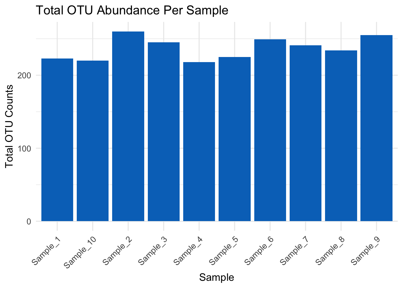
Before diving into deeper microbiome comparisons, it’s helpful to visualize the sequencing depth — the total number of OTU counts per sample. This allows you to check: - Sample variability - Potential outliers - Overall library size distribution

Using modern tools like ggplot2 in R or seaborn in Python helps create clearer, more elegant plots.

7.2 Python Code

import pandas as pd
import seaborn as sns
import matplotlib.pyplot as plt

# Load OTU table
otu_df = pd.read_csv("data/otu_table_filtered.tsv", sep="\t", index_col=0)

# Prepare data
total_counts = otu_df.sum(axis=0).reset_index()
total_counts.columns = ["Sample", "Total_OTUs"]

# Plot
plt.figure(figsize=(10, 5))
sns.barplot(data=total_counts, x="Sample", y="Total_OTUs", palette="viridis")
plt.title("Total OTU Abundance Per Sample")
plt.xticks(rotation=45)
plt.ylabel("Total OTU Counts")
plt.tight_layout()
plt.show()

7.3 R Code

library(tidyverse)

otu_df <- read.delim("data/otu_table_filtered.tsv", row.names = 1)
otu_long <- colSums(otu_df) %>%
  enframe(name = "Sample", value = "Total_OTUs")

ggplot(otu_long, aes(x = Sample, y = Total_OTUs)) +
  geom_col(fill = "#0073C2FF") +
  labs(title = "Total OTU Abundance Per Sample", y = "Total OTU Counts") +
  theme_minimal(base_size = 13) +
  theme(axis.text.x = element_text(angle = 45, hjust = 1))