Data Structure and Prevalence

Data structure and prevalence

Microbiome count data is structurally sparse and uneven.

This chapter focuses on:

Matrix sparsity
Library size variation
Taxa prevalence

Load data

ps <- readRDS("data/moving-pictures-ps.rds")

Sparsity

otu <- methods::as(phyloseq::otu_table(ps), "matrix")
if (!phyloseq::taxa_are_rows(ps)) {
  otu <- t(otu)
}

zero_prop <- mean(otu == 0)
zero_prop

[1] 0.9111154

A high proportion of zeros is normal in microbiome data.

Filtering decisions are not cosmetic. They determine which patterns become visible.

Library size variation

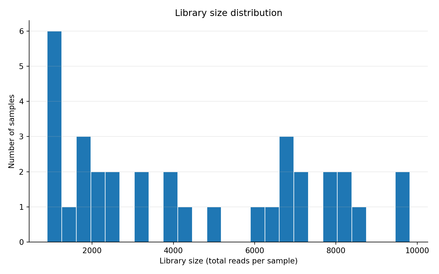
lib_size <- phyloseq::sample_sums(ps)
summary(lib_size)

   Min. 1st Qu.  Median    Mean 3rd Qu.    Max. 
    897    1838    4010    4524    7013    9820

df_lib <- data.frame(
  sample_id = names(lib_size),
  library_size = as.numeric(lib_size),
  stringsAsFactors = FALSE
)

dir.create("outputs/tables", recursive = TRUE, showWarnings = FALSE)
readr::write_csv(df_lib, "outputs/tables/library-size.csv")

Library size distribution (Python)

import pandas as pd
import matplotlib.pyplot as plt

df = pd.read_csv("outputs/tables/library-size.csv")

fig, ax = plt.subplots(figsize=(8, 5))
ax.hist(df["library_size"], bins=25, edgecolor="white", linewidth=0.8)

ax.set_title("Library size distribution")
ax.set_xlabel("Library size (total reads per sample)")
ax.set_ylabel("Number of samples")

ax.grid(True, axis="y", alpha=0.25)
ax.spines["top"].set_visible(False)
ax.spines["right"].set_visible(False)

fig.tight_layout()
plt.show()

When sequencing depth varies, raw counts are not comparable.

Normalization is required for fair comparison across samples.

Detection and prevalence

detection <- 1

taxa_prev_n <- rowSums(otu >= detection)
taxa_prev_df <- data.frame(
  taxon = rownames(otu),
  prevalence_n = taxa_prev_n,
  prevalence_frac = taxa_prev_n / ncol(otu),
  stringsAsFactors = FALSE
)

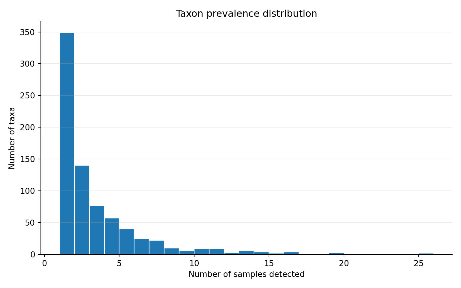
summary(taxa_prev_df$prevalence_n)

   Min. 1st Qu.  Median    Mean 3rd Qu.    Max. 
  1.000   1.000   2.000   3.022   4.000  26.000

dir.create("outputs/tables", recursive = TRUE, showWarnings = FALSE)
readr::write_csv(taxa_prev_df, "outputs/tables/taxa-prevalence.csv")

Prevalence distribution (Python)

import pandas as pd
import numpy as np
import matplotlib.pyplot as plt

df = pd.read_csv("outputs/tables/taxa-prevalence.csv")

fig, ax = plt.subplots(figsize=(8, 5))
ax.hist(df["prevalence_n"], bins=25, edgecolor="white", linewidth=0.8)

ax.set_title("Taxon prevalence distribution")
ax.set_xlabel("Number of samples detected")
ax.set_ylabel("Number of taxa")

ax.grid(True, axis="y", alpha=0.25)
ax.spines["top"].set_visible(False)
ax.spines["right"].set_visible(False)

fig.tight_layout()
plt.show()

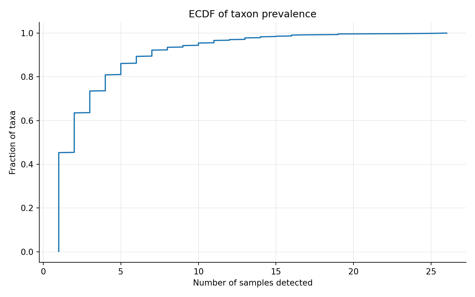
# Optional: ECDF view (often clearer for sparse data)
x = np.sort(df["prevalence_n"].to_numpy())
y = np.arange(1, len(x) + 1) / len(x)

fig, ax = plt.subplots(figsize=(8, 5))
ax.plot(x, y)
ax.set_title("ECDF of taxon prevalence")
ax.set_xlabel("Number of samples detected")
ax.set_ylabel("Fraction of taxa")

ax.grid(True, alpha=0.25)
ax.spines["top"].set_visible(False)
ax.spines["right"].set_visible(False)

fig.tight_layout()
plt.show()

Most taxa are observed in only a small fraction of samples.

Prevalence filtering improves clarity, but it also changes the feature space. Filtering rules must be stated explicitly.

Simple prevalence filter

min_prev_frac <- 0.10

keep_taxa <- taxa_prev_df$taxon[taxa_prev_df$prevalence_frac >= min_prev_frac]
ps_prev <- phyloseq::prune_taxa(keep_taxa, ps)

c(original_taxa = phyloseq::ntaxa(ps), after_filter = phyloseq::ntaxa(ps_prev))

original_taxa  after_filter 
          770           204

Prevalence filtering reduces dimensionality and improves readability.

It can also change ordination and diversity results. Interpretation should acknowledge these choices.

Relative abundance preview

ps_rel <- phyloseq::transform_sample_counts(ps, function(x) x / sum(x))
range(phyloseq::sample_sums(ps_rel))

[1] 1 1

After transformation, each sample sums to 1.

This enables clearer visualization, but does not remove compositional constraints.