ps <- readRDS("data/moving-pictures-ps.rds")

source("scripts/R/cdi-plot-theme.R")
pal <- cdi_palette()Diversity Analysis
Alpha diversity summaries are common in microbiome studies.
They are useful, but only when interpreted carefully.
This chapter focuses on:
- what alpha diversity measures
- how sequencing depth affects diversity
- how to interpret group differences responsibly
Load data
Check sequencing depth
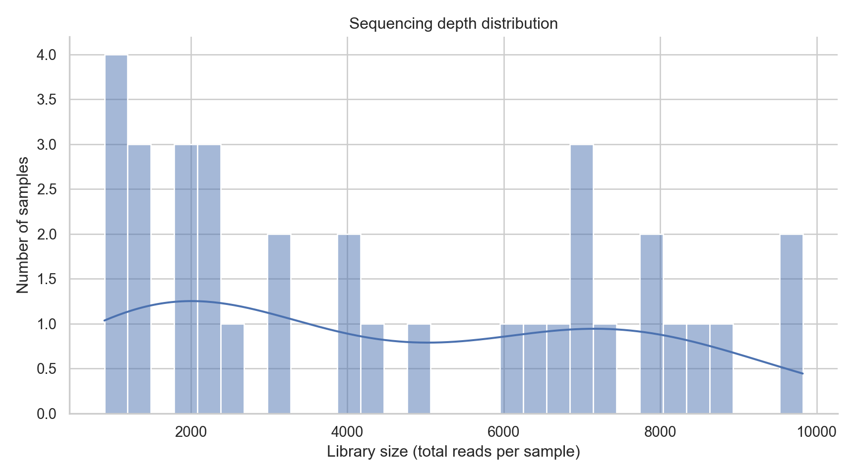
Sequencing depth varies across samples. This affects detection of rare taxa and can influence alpha diversity.
lib_size <- phyloseq::sample_sums(ps)

lib_df <- data.frame(
  sample_id = names(lib_size),
  library_size = as.numeric(lib_size),
  stringsAsFactors = FALSE
)

dir.create("outputs/tables", recursive = TRUE, showWarnings = FALSE)
readr::write_csv(lib_df, "outputs/tables/library-size.csv")ggplot2::ggplot(lib_df, ggplot2::aes(x = library_size)) +
cdi_geom_histogram(bins = 25, colored = FALSE) +
ggplot2::labs(
title = "Sequencing depth distribution",
subtitle = "Library size varies across samples",
x = "Library size (total reads per sample)",
y = "Number of samples"
) +
cdi_theme() +
ggplot2::theme(
legend.position = "none"
)
Compute alpha diversity
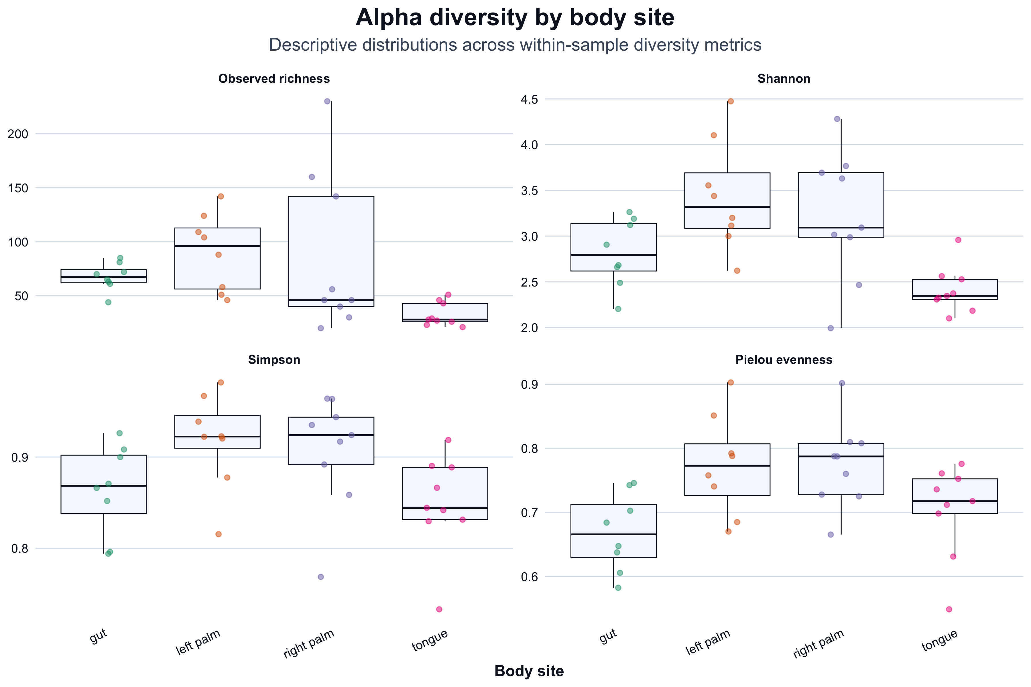
We compute four common metrics:
- Observed richness: number of detected taxa
- Shannon: richness plus evenness
- Simpson: dominance-weighted diversity
- Pielou: evenness derived from Shannon
otu <- methods::as(phyloseq::otu_table(ps), "matrix")

if (!phyloseq::taxa_are_rows(ps)) {
  otu <- t(otu)
}

observed <- colSums(otu > 0)
shannon  <- vegan::diversity(t(otu), index = "shannon")
simpson  <- vegan::diversity(t(otu), index = "simpson")
pielou   <- shannon / log(pmax(observed, 1))

alpha_df <- data.frame(
  sample_id = colnames(otu),
  observed  = as.numeric(observed),
  shannon   = as.numeric(shannon),
  simpson   = as.numeric(simpson),
  pielou    = as.numeric(pielou),
  stringsAsFactors = FALSE
)

meta <- data.frame(phyloseq::sample_data(ps))
meta$sample_id <- rownames(meta)

alpha_df <- merge(alpha_df, meta, by = "sample_id", all.x = TRUE)

cols <- names(alpha_df)
body_col <- intersect(c("body-site", "body.site", "body_site"), cols)

if (length(body_col) == 0) {
  stop(
    "Body site column not found. Available columns: ",
    paste(cols, collapse = ", ")
  )
}

alpha_df$body_site <- as.character(alpha_df[[body_col[1]]])
alpha_df <- alpha_df[!is.na(alpha_df$body_site) & alpha_df$body_site != "", , drop = FALSE]
Save alpha diversity table (for reproducibility)
dir.create("outputs/tables", recursive = TRUE, showWarnings = FALSE)
readr::write_csv(alpha_df, "outputs/tables/alpha-diversity.csv")
Alpha diversity by body site
We visualize metrics by body site as a descriptive summary.
alpha_long <- tidyr::pivot_longer(
  alpha_df,
  cols = c("observed", "shannon", "simpson", "pielou"),
  names_to = "metric",
  values_to = "value"
)

alpha_long$metric <- factor(
  alpha_long$metric,
  levels = c("observed", "shannon", "simpson", "pielou"),
  labels = c("Observed richness", "Shannon", "Simpson", "Pielou evenness")
)ggplot2::ggplot(alpha_long, ggplot2::aes(x = body_site, y = value)) +
ggplot2::geom_boxplot(
fill = pal$bg,
color = pal$ink,
linewidth = 0.35,
outlier.shape = NA
) +
ggplot2::geom_jitter(
ggplot2::aes(color = body_site),
width = 0.18,
height = 0,
alpha = 0.50,
size = 1.7,
show.legend = FALSE
) +
ggplot2::facet_wrap(~ metric, scales = "free_y", ncol = 2) +
ggplot2::labs(
title = "Alpha diversity by body site",
subtitle = "Descriptive distributions across within-sample diversity metrics",
x = "Body site",
y = NULL
) +
ggplot2::scale_color_brewer(palette = "Dark2") +
cdi_theme() +
ggplot2::theme(
axis.text.x = ggplot2::element_text(angle = 25, hjust = 1),
legend.position = "none"
)
Interpretation reminder
This guide is descriptive. It shows what the data look like and how common summaries behave.
To make inferential claims, you would typically add:
- statistical testing under appropriate assumptions
- covariate handling (confounding, repeated measures)
- multivariate modeling for community-level change
Those topics belong in the premium continuation.